Calibrating Algorithm Throughput & Generating Contrast Curves
Due to oversubtraction and selfsubtraction (see Pueyo (2016) for a good explaination), the shape, flux, and spectrum of the signal of a planet or disk is distoed by PSF subtraction. To calibrate algorithm throughput after KLIP in this tutorial, we will use the standard fake injection technique, which basically is injecting fake planets/disks in the data of known shape, flux, and spectrum to measure the algorithm throughput.
In this tutorial, we will calibrate the throughput of the previous exmaple (Basic KLIP Tutorial with GPI) for the purpose of generating a contrast curve. Note that this same general process can be used to character a planet or disk (e.g. measure astrometry and spectrum of an imaged exoplanet).
Contrast Curves
To measure the contrast (ignoring algorithm throughput), we use pyklip.klip.meas_contrast(), which assumes
azimuthally symmetric noise and computes the 5σ noise level at each separation. It uses a Gaussian cross correlation to
compute the noise as a small optimization to smooth out high frequency noise (since we know our planet is not going to
be smaller than on λ/D scales). It also corrects for small number statistics (i.e. by assuming a Student’s
t-distribution rather than a Gaussian).
This will give us a sense of the contrast to inject fake planets into the data (algorithm throughput is ~50%).
We are calculating broadband contrast so we want to spectrally-collapsed data (if applicable). You can do this
by reading back in the KL mode cube and picking a KL mode cutoff. (The KL mode cutoff is chosen to maximize planet SNR, which we won’t discuss here, but can be determined with fake planet injection.)
Here we will show an example using the pyKLIP output of GPI data, and using KL modes.
import astropy.io.fits as fits
hdulist = fits.open("myobject-KLmodes-all.fits")
# pick the 20 KL mode cutoff frame out of [1,20,50,100]
kl20frame = hdulist[1].data[1]
dataset_center = [hdulist[1].header['PSFCENTX'], hdulist[1].header['PSFCENTY'] ]
Then, a convenient pyKLIP function will calculate the contrast, accounting for small sample statistics. We are picking 1.1 arcseconds as the outer boundary of our contrast curve. The low_pass_filter option specifies the size of the Gaussian to use in our cross correlation to smooth low frequency noise. It is typically smaller than the size of the PSF since self-subtraction from KLIP decreases the PSF size. We also need to specify the FWHM of the PSF in order to account for small sample statistics. It also determines the spacing the contrast curve returns. The function samples the noise with a spacing of FWHM/2.
For our example dataset on Beta Pic, we also need to mask out the planet, Beta Pic b, so that it doesn’t bias our noise estimate.
import numpy as np
import pyklip.klip as klip
import pyklip.instruments.GPI as GPI

dataset_iwa = GPI.GPIData.fpm_diam['J']/2 # radius of occulter
dataset_owa = 1.5/GPI.GPIData.lenslet_scale # 1.5" is the furtherest out we will go
dataset_fwhm = 3.5 # fwhm of PSF roughly
low_pass_size = 1. # pixel, corresponds to the sigma of the Gaussian

# mask beta Pic b
# first get the location of the planet from Wang+ (2016)
betapicb_sep = 30.11 # pixels
betapicb_pa = 212.2 # degrees
betapicb_x = betapicb_sep * -np.sin(np.radians(betapicb_pa)) + dataset_center[0]
betapicb_y = betapicb_sep * np.cos(np.radians(betapicb_pa)) + dataset_center[1]
# now mask the data
ydat, xdat = np.indices(kl20frame.shape)
distance_from_planet = np.sqrt((xdat - betapicb_x)**2 + (ydat - betapicb_y)**2)
kl20frame[np.where(distance_from_planet <= 2*dataset_fwhm)] = np.nan


contrast_seps, contrast = klip.meas_contrast(kl20frame, dataset_iwa, dataset_owa, dataset_fwhm, center=dataset_center, low_pass_filter=low_pass_size)
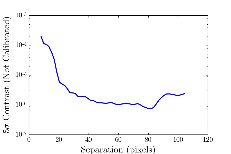
Now we can plot what the contrast curve (missing a calibration for algorithm throughput) looks like.
Injecting Fake Planets
KLIP naturally subtracts out planet flux due to over-subtraction and self-subtraction. To calibrate our sensitivity to planets, we need to inject some fake planets at known brightness into our data to calibrate KLIP attenuation. In this tutorial, we only only inject a few fakes once into the data just to demonstrate the technique with pyKLIP. For your data, it is suggested you inject many planets to explore the attenuation factor as a function of brightness, separation, and KLIP parameters (more aggressive reductions increase attenuation of flux due to KLIP).Fake planets are free, so the more the merrier!
First, let’s read in the data again. This is the same dataset as you read in to run KLIP the first time.
import glob

filelist = glob.glob("path/to/dataset/*.fits")
dataset = GPI.GPIData(filelist, highpass=True)
Now we’ll inject 12 fake planets in each cube. We’ll do this one fake planet at a time using pyklip.fakes.inject_planet(). As we get further out in the image, we will inject fainter planets, since the throughput does vary with planet flux, so we want the fake planets to be just around the detection threshold (slightly above is preferably to reduce noise). Since we specify a fake planet’s location by it’s separation and position angle, we need to know the orientation of the sky on the image using the frames’ WCS headers. The planets also are injected in raw data units, we need to convert the planet flux from contrast to DN for GPI. For other instruments, each should have its flux calibration and thus own method to convert between data units and contrast.
import pyklip.fakes as fakes

# three sets, planets get fainter as contrast gets better further out
input_planet_fluxes = [1e-4, 1e-5, 5e-6]
seps = [20, 40, 60]
fwhm = 3.5 # pixels, approximate for GPI

for input_planet_flux, sep in zip(input_planet_fluxes, seps):
    # inject 4 planets at that separation to improve noise
    # fake planets are injected in data number, not contrast units, so we need to convert the flux
    # for GPI, a convenient field dn_per_contrast can be used to convert the planet flux to raw data numbers
    injected_flux = input_planet_flux * dataset.dn_per_contrast
    for pa in [0, 90, 180, 270]:
        fakes.inject_planet(dataset.input, dataset.centers, injected_flux, dataset.wcs, sep, pa, fwhm=fwhm)
Now we’ll run KLIP using the example same parameters on this dataset with fake planets.
import pyklip.parallelized as parallelized

parallelized.klip_dataset(dataset, outputdir="path/to/save/dir/", fileprefix="myobject-withfakes",
                          annuli=9, subsections=4, movement=1, numbasis=[1,20,50,100],
                          calibrate_flux=True, mode="ADI+SDI")
Now, the resulting KLIP dataset should have 12 more planets in it! For the Beta Pic dataset, we actually have 13 planets ;).
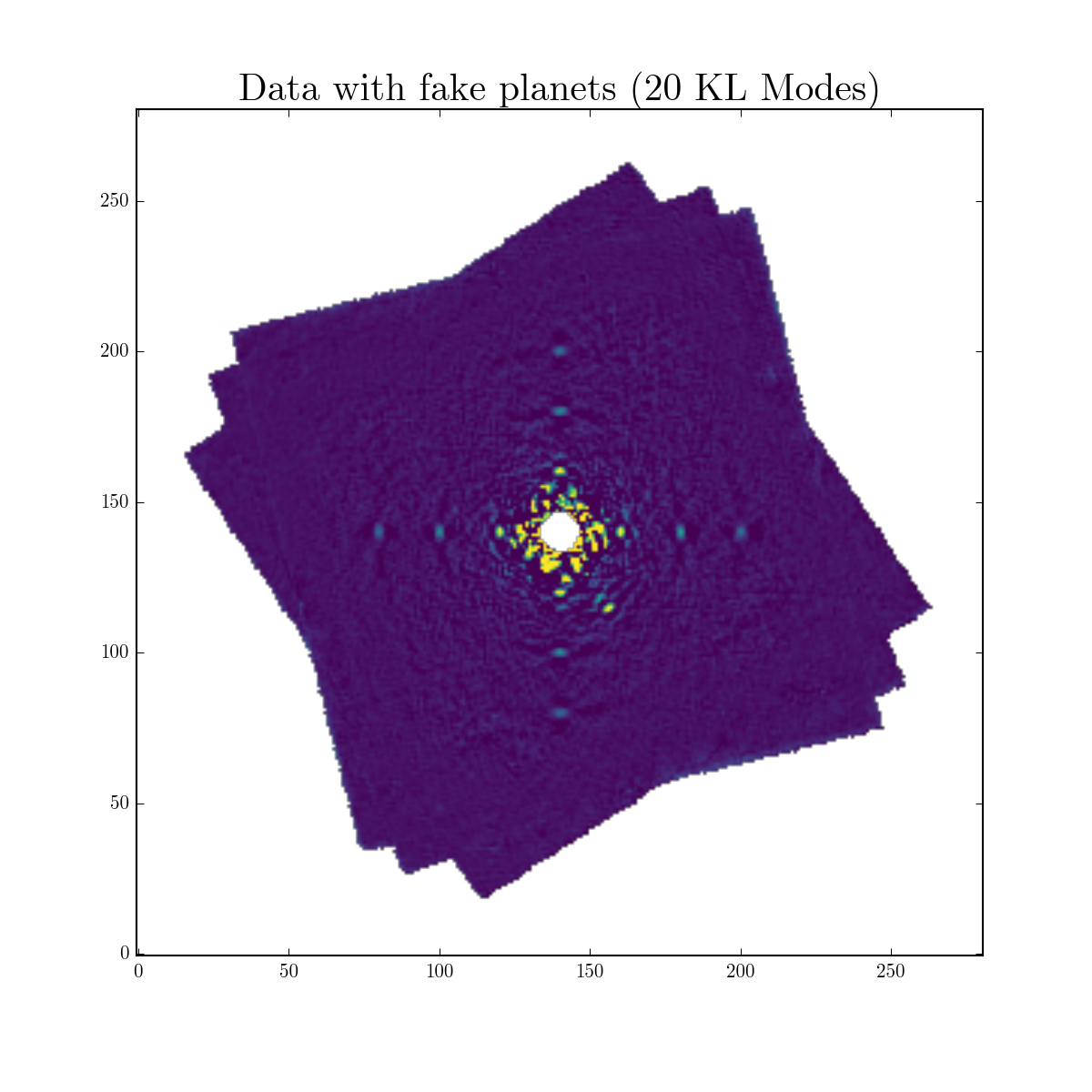
We now will read in the output of the KLIP reducation with fake planets. Since we’re using the 20 KL mode cutoff frame for our contrast curve, we want the same cutoff for our reduction with fake planets.
kl_hdulist = fits.open("myobject-withfakes-KLmodes-all.fits")
dat_with_fakes = kl_hdulist[1].data[1]
dat_with_fakes_centers = [kl_hdulist[1].header['PSFCENTX'], kl_hdulist[1].header['PSFCENTY'] ]
We will measure the flux of each fake in the reduced image using pyklip.fakes.retrieve_planet_flux(). Our strategy here is to assume the throughput is constant azimuthally, and for each 4 planets at a separation, average their fluxes together to reduce noise. Note that we need to again specify a WCS header (the one corresponding to the output images) to tell the code where to look for the planet in the image. You can grab that from the header of the reduced image, or we will be lazy here are use the dataset.output_wcs field from our fake dataset, which automatically gets rotated after KLIP.
retrieved_fluxes = [] # will be populated, one for each separation

for input_planet_flux, sep in zip(input_planet_fluxes, seps):
    fake_planet_fluxes = []
    for pa in [0, 90, 180, 270]:
        fake_flux = fakes.retrieve_planet_flux(dat_with_fakes, dat_with_fakes_centers, dataset.output_wcs[0], sep, pa, searchrad=7)
        fake_planet_fluxes.append(fake_flux)
    retrieved_fluxes.append(np.mean(fake_planet_fluxes))
Now we can calibrate the contrast curves. We know what flux level we injected the planets into the data at. We now have measured the flux value of the planets at each separation, so we can now calculate the “algorithm throughput” which measures how much KLIP attenuates flux. Then for each location on the contrast curve, we will just use the closest fake planet injection separation to assume an algorithm throughput correction. This is why it is good in practice in inject fakes in as many places as possible, so that the fake planets better model the algorithm throughput at each separation.
# fake planet output / fake planet input = throughput of KLIP
algo_throughput = np.array(retrieved_fluxes)/np.array(input_planet_fluxes) # a number less than 1 probably

corrected_contrast_curve = np.copy(contrast)
for i, sep in enumerate(contrast_seps):
    closest_throughput_index = np.argmin(np.abs(sep - seps))
    corrected_contrast_curve[i] /= algo_throughput[closest_throughput_index]
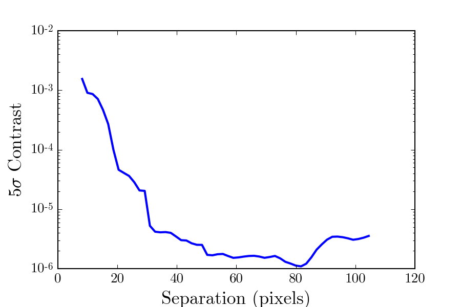
Finally, we get a calibrated contrast curve!
Coronagraphic Throughput
If a coronagraph was used in data collection, it can have a measurable effect on the planet fluxes that we’re able to detect. Closer to the star, we might expect a coronograph to cause major dimming of observed planets, while planets at further separations from the star will likely be unaffected. Each coronagraph will typically have its own transmission profile, a measure of how its throughput changes as a function of distance from the center. It is quite useful for us to incorporate this into our contrast measurements in order to get a more accurate estimation of how bright planets must be in order for us to find them. Luckily, we can account for this coronagraphic effect on light transmission while estimating pyKLIP’s equivalent effect on planet flux, thereby jointly calibrating both coronagraphic and algorithmic throughput. The following will explain how we integrate the coronagraphic throughput correction by making a small modification to our fake planet injection function.
The pyklip.fakes.inject_planet() function has an optional argument field_dependent_correction, which accepts
a user provided function that corrects for coronagraphic throughput. The provided function should accept three arguments: the region or ‘stamp’ of your fake planet,
the physical ‘x’ separation of each pixel in the stamp from the center, and the physical ‘y’ separation of each pixel in the stamp from the center.
Provided with the transmission profile of the relevant coronagraph, this function should then scale the input stamp by the necessary amount, then output the throughput corrected stamp.
Prior to creating the function, be sure to read in your coronagraphic transmission profile. This should include columns for the transmission and distance from the star (in pixels).
# Read in transmission profile first

def transmission_correction(input_stamp, input_dx, input_dy):
    """
    Args:
        input_stamp (array): 2D array of the region surrounding the fake planet injection site
        input_dx (array): 2D array specifying the x distance of each stamp pixel from the center
        input_dy (array): 2D array specifying the y distance of each stamp pixel from the center

    Returns:
        output_stamp (array): 2D array of the throughput corrected planet injection site.
    """
    # Calculate the distance of each pixel in the input stamp from the center
    distance_from_center = np.sqrt((input_dx)**2+(input_dy)**2)

    # Select the relevant columns from the coronagraph's transmission profile
    transmission =  transmission_profile['throughput']
    radius = transmission_profile['distance']

    # Interpolate to find the transmission value for each pixel in the input stamp
    transmission_of_stamp = np.interp(distance_from_center, radius, transmission)

    # Reshape the interpolated array to have the same dimensions as the input stamp
    transmission_of_stamp = transmission_of_stamp.reshape(input_stamp.shape)

    # Make the throughput correction
    output_stamp = transmission_of_stamp*input_stamp

    return output_stamp
Now, we can include the function as an optional argument in pyklip.fakes.inject_planet():
import pyklip.fakes as fakes

# three sets, planets get fainter as contrast gets better further out
input_planet_fluxes = [1e-4, 1e-5, 5e-6]
seps = [20, 40, 60]
fwhm = 3.5 # pixels, approximate for GPI

for input_planet_flux, sep in zip(input_planet_fluxes, seps):
    # inject 4 planets at that separation to improve noise
    # fake planets are injected in data number, not contrast units, so we need to convert the flux
    # for GPI, a convenient field dn_per_contrast can be used to convert the planet flux to raw data numbers
    injected_flux = input_planet_flux * dataset.dn_per_contrast
    for pa in [0, 90, 180, 270]:
        fakes.inject_planet(dataset.input,
                            dataset.centers,
                            injected_flux,
                            dataset.wcs,
                            sep,
                            pa,
                            fwhm=fwhm,
                            field_dependent_correction = transmission_correction)