Foward-Model Astrometry and Photometry

pyKLIP offers PSF fitting as the most optimal method for extraction of planet astrometry and photometry. Astrometry/photometry of directly imaged exoplanets is challenging since PSF subtraction algorithms (like pyKLIP) distort the PSF of the planet. Pueyo (2016) provide a technique to forward model the PSF of a planet through KLIP. Taking this forward model, you could fit it to the data, but you would underestimate your errors because the noise in direct imaging data is correlated (i.e. each pixel is not independent). To account for the correlated nature of the noise, we use Gaussian process regression to model and account for the correlated nature of the noise. This allows us to obtain accurate measurements and accurate uncertainties on the planet parameters.

The code was originally designed for the Bayesian KLIP-FM Astorometry technique (BKA) that is described in Wang et al. (2016) to obtain one milliarcsecond astrometry on β Pictoris b. Since then, it has be extended to also do maximum likelihood fitting in a frequentist framework that can also obtain uncertainties. A frequentist framework is appropriate when astrometric calibration uncertainties are also derived in a frequentist procedure.

Attribution

If you use this feature, please cite:

• Wang, J. J., Graham, J. R., Pueyo, L., et al. 2016, AJ, 152, 97.

• Pueyo, L. 2016, ApJ, 824, 117.

If you used the MCMC sampling aspects of this feature, please cite:

• Foreman-Mackey, D., Hogg, D. W., Lang, D., et al. 2013, PASP, 125, 306.

Requirements

You need the following pieces of data to forward model the data. (If you have a model and some data to fit to, you can skip the section on using KLIP-FM to generate a forawrd model PSF.)

• Data to run PSF subtraction on

• A model or data of the instrumental PSF

• A good guess of the position of the planet (a center of light centroid routine should get the astrometry to a pixel)

• For IFS data, an estimate of the spectrum of the planet (it does not need to be very accurate, and 20% errors are fine)

If you want to run BKA, you need the additional packages installed, which should be available readily:

• emcee

• corner

Generating instrumental PSFs for GPI

A quick aside for GPI spectral mode data, here is how to generate the instrumental PSF from the satellite spots.

import glob
import numpy as np
import pyklip.instruments.GPI as GPI

# read in the data into a dataset
filelist = glob.glob("path/to/dataset/*.fits")
dataset = GPI.GPIData(filelist)

# generate instrumental PSF
boxsize = 17 # we want a 17x17 pixel box centered on the instrumental PSF
dataset.generate_psfs(boxrad=boxsize//2) # this function extracts the satellite spots from the data
# now dataset.psfs contains a 37x25x25 spectral cube with the instrumental PSF
# normalize the instrumental PSF so the peak flux is unity
dataset.psfs /= (np.mean(dataset.spot_flux.reshape([dataset.spot_flux.shape[0] // 37, 37]),
                         axis=0)[:, None, None])

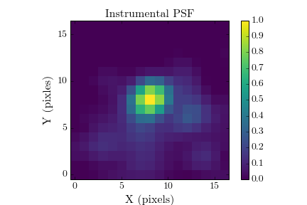
Here is an exmaple using three datacubes from the publicly available GPI data on beta Pic. Note that the wings of the PSF are somewhat noisy, due to the fact the speckle noise in J-band is high near the satellite spots. However, this should still give us an acceptable instrumental PSF.

Forward Modelling the PSF with KLIP-FM

With an estimate of the planet position, the instrumental PSF, and, if applicable, an estimate of the spectrum, we can use the pyklip.fm implementation of KLIP-FM and pyklip.fmlib.fmpsf.FMPlanetPSF extension to forward model the PSF of a planet through KLIP.

First, let us initalize pyklip.fmlib.fmpsf.FMPlanetPSF to forward model the planet in our data.

For GPI, we are using normalized copies of the satellite spots as our input PSFs, and because of that, we need to pass in a flux conversion value, dn_per_contrast, that allows us to scale our guessflux in contrast units to data units. If you are not using normalized PSFs, dn_per_contrast should be the factor that scales your input PSF to the flux of the unocculted star. If your input PSF is already scaled to the flux of the stellar PSF, dn_per_contrast is optional and should not actually be passed into the function.

# setup FM guesses
# You should change these to be suited to your data!
numbasis = np.array([1, 7, 100]) # KL basis cutoffs you want to try
guesssep = 30.1 # estimate of separation in pixels
guesspa = 212.2 # estimate of position angle, in degrees
guessflux = 5e-5 # estimated contrast
dn_per_contrast = your_flux_conversion # factor to scale PSF to star PSF. For GPI, this is dataset.dn_per_contrast
guessspec = your_spectrum # should be 1-D array with number of elements = np.size(np.unique(dataset.wvs))

# initialize the FM Planet PSF class
import pyklip.fmlib.fmpsf as fmpsf
fm_class = fmpsf.FMPlanetPSF(dataset.input.shape, numbasis, guesssep, guesspa, guessflux, dataset.psfs,
                             np.unique(dataset.wvs), dn_per_contrast, star_spt='A6',
                             spectrallib=[guessspec])

Note

When executing the initializing of FMPlanetPSF, you will get a warning along the lines of “The coefficients of the spline returned have been computed as the minimal norm least-squares solution of a (numerically) rank deficient system.” This is completely normal and expected, and should not be an issue.

Next we will run KLIP-FM with the pyklip.fm module. Before we run it, we will need to pick our PSF subtraction parameters (see the Basic KLIP Tutorial with GPI for more details on picking KLIP parameters). For our zones, we will run KLIP only on one zone: an annulus centered on the guessed location of the planet with a width of 30 pixels. The width just needs to be big enough that you see the entire planet PSF.

# PSF subtraction parameters
# You should change these to be suited to your data!
outputdir = "." # where to write the output files
prefix = "betpic-131210-j-fmpsf" # fileprefix for the output files
annulus_bounds = [[guesssep-15, guesssep+15]] # one annulus centered on the planet
subsections = 1 # we are not breaking up the annulus
padding = 0 # we are not padding our zones
movement = 4 # we are using an conservative exclusion criteria of 4 pixels

# run KLIP-FM
import pyklip.fm as fm
fm.klip_dataset(dataset, fm_class, outputdir=outputdir, fileprefix=prefix, numbasis=numbasis,
                annuli=annulus_bounds, subsections=subsections, padding=padding, movement=movement)

This will now run KLIP-FM, producing both a PSF subtracted image of the data and a forward-modelled PSF of the planet at the gussed location of the planet. The PSF subtracted image as the “-klipped-” string in its filename, while the forward-modelled planet PSF has the “-fmpsf-” string in its filename.

Fitting the Planet PSF

Now that we have the forward-modeled PSF and the data, we can fit the model PSF to the data and obtain the astrometry/photometry of the point source. To do it the Bayesian way with MCMC or the frequentist way with maximum likelihood is very similar in the code, and will produce similar results as both frameworks use the forward-modeled PSF and Gaussian process regression. The difference is interpretation, and determining which framework makes sense for your analysis (e.g., if the instrument calibration was done in a Bayesian sense, then doing the fit in a Bayesian way is appropriate to properly combine calibration uncertainties with measurement uncertainties).

First, let’s read in the data from our previous forward modelling. We will take the collapsed KL mode cubes, and select the KL mode cutoff we want to use. For the example, we will use 7 KL modes to model and subtract off the stellar PSF.

import os
import astropy.io.fits as fits
# read in outputs
output_prefix = os.path.join(outputdir, prefix)
fm_hdu = fits.open(output_prefix + "-fmpsf-KLmodes-all.fits")
data_hdu = fits.open(output_prefix + "-klipped-KLmodes-all.fits")

# get FM frame, use KL=7
fm_frame = fm_hdu[1].data[1]
fm_centx = fm_hdu[1].header['PSFCENTX']
fm_centy = fm_hdu[1].header['PSFCENTY']

# get data_stamp frame, use KL=7
data_frame = data_hdu[1].data[1]
data_centx = data_hdu[1].header["PSFCENTX"]
data_centy = data_hdu[1].header["PSFCENTY"]

# get initial guesses
guesssep = fm_hdu[0].header['FM_SEP']
guesspa = fm_hdu[0].header['FM_PA']

We will generate a pyklip.fitpsf.FMAstrometry object that will handle all of the fitting processes. The first thing we will do is create this object, and feed it in the data and forward model. It will use them to generate stamps of the data and forward model which can be accessed using fit.data_stmap and fit.fm_stamp respectively. When reading in the data, it will also generate a noise map for the data stamp by computing the standard deviation around an annulus, with the planet masked out. Here, we will also specify whether we will use a maximum likliehood or MCMC technique to derive the best-fit and uncertainties using the argument method="mcmc" (default) or method="maxl".

import pyklip.fitpsf as fitpsf
# create FM Astrometry object that does MCMC fitting
fit = fitpsf.FMAstrometry(guesssep, guesspa, 13, method="mcmc")
# alternatively, could use maximum likelihood fitting
# fit = fitpsf.FMAstrometry(guesssep, guesspa, 13, method="maxl")

# generate FM stamp
# padding should be greater than 0 so we don't run into interpolation problems
fit.generate_fm_stamp(fm_frame, [fm_centx, fm_centy], padding=5)

# generate data_stamp stamp
# not that dr=4 means we are using a 4 pixel wide annulus to sample the noise for each pixel
# exclusion_radius excludes all pixels less than that distance from the estimated location of the planet
fit.generate_data_stamp(data_frame, [data_centx, data_centy], dr=4, exclusion_radius=10)

Next we need to choose a Gaussian process kernel to model the correlated noise in our data. We currently only support the Matern (ν=3/2) and square exponential kernel, so we will pick the Matern kernel here. Note that there is the option to add a diagonal (i.e. read/photon noise) term to the kernel, but we have chosen not to use it in this example. If you are not dominated by speckle noise (i.e. around fainter stars or further out from the star), you should enable the read noies term.

# set kernel, no read noise
corr_len_guess = 3.
corr_len_label = r"$l$"
fit.set_kernel("matern32", [corr_len_guess], [corr_len_label])

MCMC takes a Bayesian approach to estimating our parameters of interest by approximating their posterior distributions i.e. their best fit values given the data. In order to perform this type of Bayesian analysis you will need to define priors, which are your own estimations of what these parameter values might be. Since we usually don’t know much about the data, we will use uniform priors, essentially estimating the same probability for each value. All we will need to specify in this case are the bounds/range of values to the uniform prior. This same code can also be used to specify parameter bounds for the maximum likelihood approach, but setting bounds is not required for that technique. The priors in the x/y position will be flat in linear space, and the priors on the flux scaling and kernel parameters will be flat in log space, since they are scale parameters. In the function below, we will set the boundaries of the priors. The first two values are for x/y and they basically say how far away (in pixels) from the guessed position of the planet can the chains wander. For the rest of the parameters, the values specify how many orders of magnitude the chains can go from the guessed value (e.g. a value of 1 means we allow a factor of 10 variation in the value).

# set bounds
x_range = 1.5 # pixels
y_range = 1.5 # pixels
flux_range = 1. # flux can vary by an order of magnitude
corr_len_range = 1. # between 0.3 and 30
fit.set_bounds(x_range, y_range, flux_range, [corr_len_range])

Finally, we are set up to fit to the data. The fit_astrometry() function is used for both MCMC and maximum likelihood. In this example, we will fit for four parameters. The RA offset and Dec offset are what we are interested in for the purposes of astrometry. The flux scaling paramter (α) is a multiplicative correction to guessflux for measuring the photometry. The correlation length (l) is a Gaussian process hyperparameter. If we had included read noise, it would have been a fifth parameter. As the analysis diverges, we will discuss Maximum Likelihood and Bayesian MCMC Analysis separately.

Bayesian MCMC Analysis

To run the MCMC sampler (using the emcee package), we need to specify the number of walkers (the number of Markov chains that explore your parameter space), number of steps each walker takes (how many new values of your parameter each chain should explore), and the number of production steps the walkers take (the number of steps we let each chain take to burn-in). We also can specify the number of threads to use. If you have not turned BLAS and MKL off, you probably only want one or a few threads, as MKL/BLAS automatically parallelizes the likelihood calculation, and trying to parallelize on top of that just creates extra overhead.

# run MCMC fit
fit.fit_astrometry(nwalkers=100, nburn=200, nsteps=800, numthreads=1)

fit.sampler stores the emcee.EnsembleSampler object which contains the full chains and other MCMC fitting information.

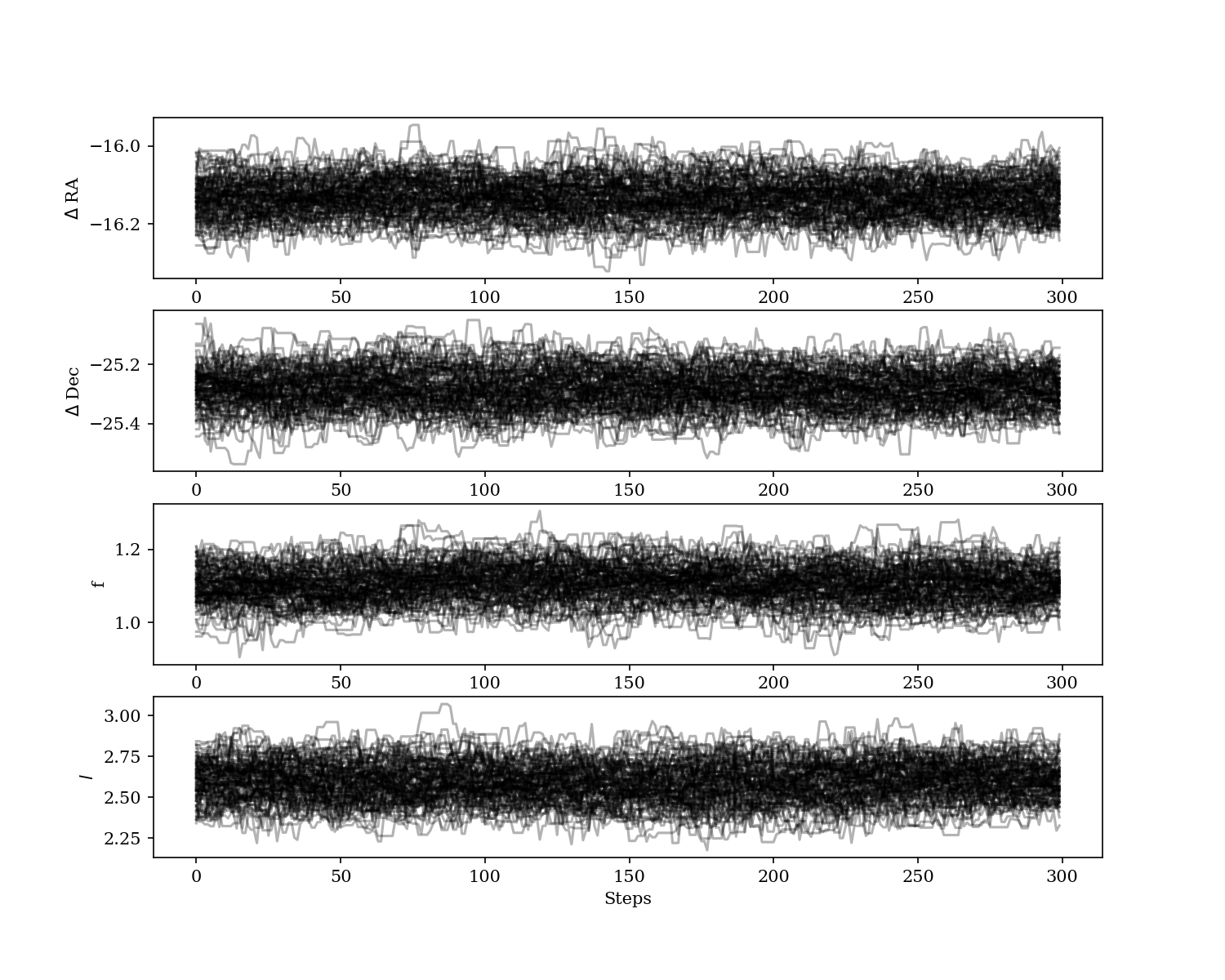
For MCMC, we want to check to make sure all of our chains have converged by plotting them. That is, we need to ensure that there are no large scale movements, and that the entire parameter space is being sampled evenly. The maximum likelihood technique skips this step.

import matplotlib.pylab as plt
fig = plt.figure(figsize=(10,8))

# grab the chains from the sampler
chain = fit.sampler.chain

# plot RA offset
ax1 = fig.add_subplot(411)
ax1.plot(chain[:,:,0].T, '-', color='k', alpha=0.3)
ax1.set_xlabel("Steps")
ax1.set_ylabel(r"$\Delta$ RA")

# plot Dec offset
ax2 = fig.add_subplot(412)
ax2.plot(chain[:,:,1].T, '-', color='k', alpha=0.3)
ax2.set_xlabel("Steps")
ax2.set_ylabel(r"$\Delta$ Dec")

# plot flux scaling
ax3 = fig.add_subplot(413)
ax3.plot(chain[:,:,2].T, '-', color='k', alpha=0.3)
ax3.set_xlabel("Steps")
ax3.set_ylabel(r"$\alpha$")

# plot hyperparameters.. we only have one for this example: the correlation length
ax4 = fig.add_subplot(414)
ax4.plot(chain[:,:,3].T, '-', color='k', alpha=0.3)
ax4.set_xlabel("Steps")
ax4.set_ylabel(r"$l$")

Here is an example using three cubes of public GPI data on beta Pic.

For MCMC, we can also plot the corner plot to look at our posterior distribution and correlation between parameters. We can use the peak of each posterior distribution to estimate the best fit value of each parameter.

fig = plt.figure()
fig = fit.make_corner_plot(fig=fig)

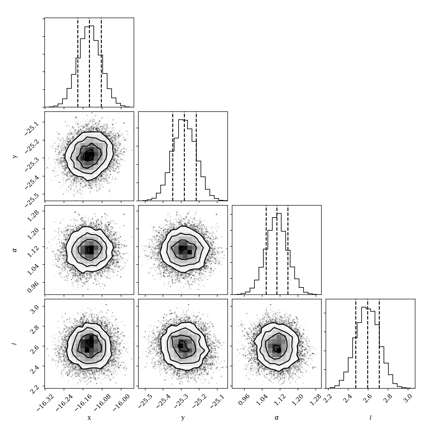
Hopefully the corner plot does not contain too much structure (the posteriors should be roughly Gaussian). In the example figure from three cubes of GPI data on beta Pic, the residual speckle noise has not been very whitened, so there is some asymmetry in the posterior, which represents the local strucutre of the speckle noise. These posteriors should become more Gaussian as we add more data and whiten the speckle noise.

To continue, skip to Output of FMAstrometry.

Maximum Likelihood

For maximum likelihood, we can start with the same FMAstrometry setup up until fit_astrometry(). The execution of fit_astrometry() will be completely different. The algorithm with use a Nelder-Mead optimization to find the global maximum, as it is a fairly robust method. Then, it will use BFGS algorithm from scipy.optimize.minimze that can approximate the Hessian inverse during the optimization. The Hessian inverse can be used as an approximation of the covariance matrix for the fitted parameters. We take the diagonal terms of the Hessian inverse as the variance in each parameter.

# if you're running a max-likelihood fit
fit.fit_astrometry()

We also store the Hessian inverse in fit.hess_inv. Note that the algorithm we use is unable to estimate the uncertainity on the Gaussian parameter hyperparameters, so those entries with all be 0.

Note

If you get a warning here about the optimizer not converging, this means that the BFGS algorithm in scipy.optimize.minimize was unable to converge on estimating the Hessian inverse, and thus the reported uncertainties are likely unreliable. We are working on a solution to this. We recommend using fake planet injection instead to estimate your uncertainities if this happens.

Output of FMAstrometry

Here are some fields to access the fit. Each field is a pyklip.fitpsf.ParamRange object, which has fields bestfit, error, and error_2sided. Here, error is the average 1-sigma error, and error_2sided lists the positive and negative errors separately. Notice the names all begin with “raw”, which is because these are the values from just fitting the data, and do not include instrument calibration.

• fit.raw_RA_offset: RA offset of the planet from the star (in pixels)

• fit.raw_Dec_offset: Dec offset of the planet from the star (in pixels)

• fit.raw_flux: Multiplicative factor to scale the model flux to match the data

• fit.covar_params: hyperparameters on the Gaussian process. This is a list with length equal to the number of hyperparameters.

Note that since fit.covar_params is a list dependent on user input, you need to index that list in order to see the bestfit values for each element. For example, fit.covar_params[0].bestfit will output the bestfit for the first element in the list.

Generally, it is good to look at the fit visually, and examine the residual plot for structure that might be indicative of a bad fit or systematics in either the data or the model.

fig = plt.figure()
fig = fit.best_fit_and_residuals(fig=fig)

And here is the example from the three frames of beta Pic b J-band GPI data:

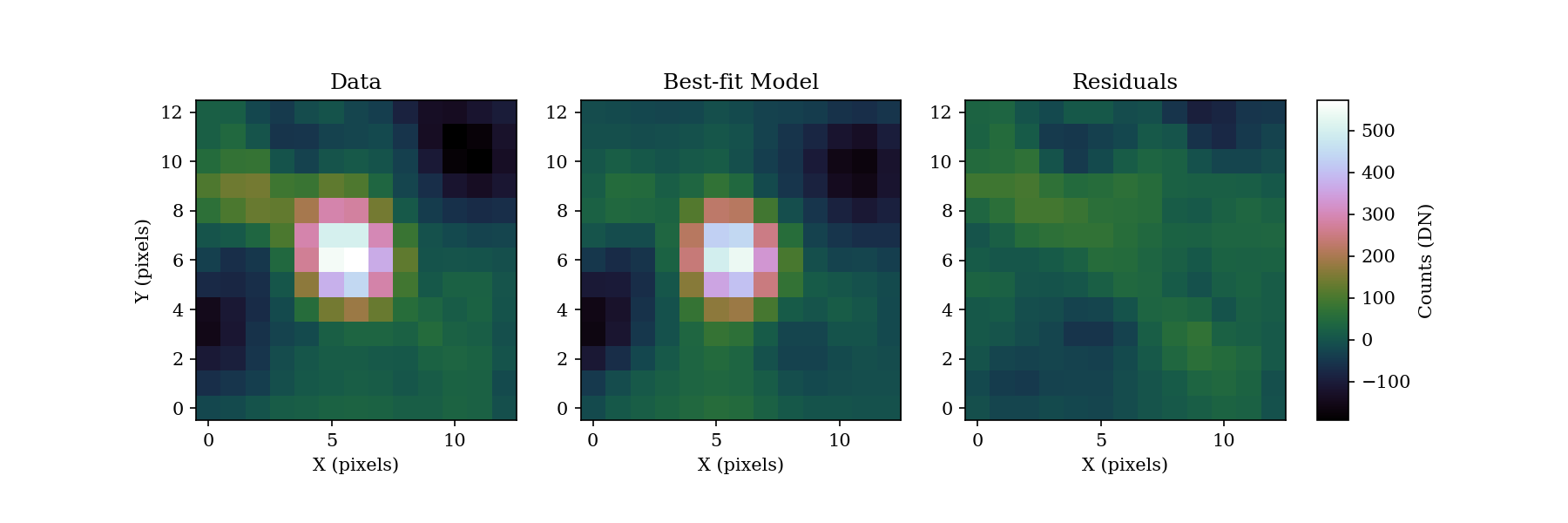
The data and best fit model should look pretty close, and the residuals hopefully do not show any obvious strcuture that was missed in the fit. The residual ampltidue should also be consistent with noise. If that is the case, we can use the best fit values for the astrometry of this epoch.

The best fit values from the MCMC give us the raw RA and Dec offsets for the planet. We will still need to fold in uncertainties in the star location and calibration uncertainties. To do this, we use pyklip.fitpsf.FMAstrometry.propogate_errs() to include these terms and obtain our final astrometric values. All of the infered parameters are fields that can be accessed (see pyklip.fitpsf.FMAstrometry) and each field is a pyklip.fitpsf.ParamRange object. Here is a brief overview of the fields:

• fit.RA_offset: RA offset of the planet from the star (angular units)

• fit.Dec_offset: Dec offset of the planet from the star (angular units)

• fit.sep: Radial separation of the planet from the star (angular units)

• fit.PA: Position angle of the planet (i.e., Angle from North towards East; in degrees).

There is currently no infrastrucutre to propogate photometric calibration uncertainities in, so it will need to be done by hand.

fit.propogate_errs(star_center_err=0.05, platescale=GPI.GPIData.lenslet_scale*1000, platescale_err=0.007, pa_offset=-0.1, pa_uncertainty=0.13)


# show what the raw uncertainites are on the location of the planet
print("\nPlanet Raw RA offset is {0} +/- {1}, Raw Dec offset is {2} +/- {3}".format(fit.raw_RA_offset.bestfit, fit.raw_RA_offset.error,
                                                                                    fit.raw_Dec_offset.bestfit, fit.raw_Dec_offset.error))

# Full error budget included
print("Planet RA offset is at {0} with a 1-sigma uncertainity of {1}".format(fit.RA_offset.bestfit, fit.RA_offset.error))
print("Planet Dec offset is at {0} with a 1-sigma uncertainity of {1}".format(fit.Dec_offset.bestfit, fit.Dec_offset.error))

# Propogate errors into separation and PA space
print("Planet separation is at {0} with a 1-sigma uncertainity of {1}".format(fit.sep.bestfit, fit.sep.error))
print("Planet PA at {0} with a 1-sigma uncertainity of {1}".format(fit.PA.bestfit, fit.PA.error))

Correcting for Coronagraphic Throughput

Coronagraphs have measurable effects on the planet fluxes that we measure. Typically, we can expect them to diminish the overall image flux at separations closer to host star, while larger separations remain relatively unaffected. In order to improve the accuracy of our forward model, pyKLIP allows users to account for this coronahgraphic effect on planet light transmission when initializing the fmpsf.FMPlanetPSF class. This feature can be accessed by providing the optional argument ‘field_dependent_correction’, which accepts a user provided function to correct for coronagraphic throughput. Each coronagraph has its own transmission profile, a measure of how its throughput changes as a function of distance from the center. As an example of how this would be incoporated, we’ll use the transmission profile of the JWST/NIRCAM MASK210 coronagraph (obtained from the Occulting Masks section of this NIRCAM webpage: https://jwst-docs.stsci.edu/near-infrared-camera/nircam-instrumentation/nircam-coronagraphic-occulting-mas

First, we’ll create a function that performs the coronagraphic throughput correction. It should accept three arguments: the region or ‘stamp’ of your fake planet, the physical ‘x’ separation of each pixel in the stamp from the coronagraph center, and the physical ‘y’ separation of each pixel in the stamp from the coronagraph center. It should then use the transmission profile of the relevant coronagraph to scale the input stamp by the necessary amount, then output the throughput corrected stamp. Be sure to read in your coronagraphic transmission profile with columns for ‘transmission’ and ‘distance from the star (in pixels)’ prior to creating the function.

# Read in transmission profile first

def transmission_correction(input_stamp, input_dx, input_dy):
    """
    Args:
        input_stamp (array): 2D array of the region surrounding the fake planet injection site
        input_dx (array): 2D array specifying the x distance of each stamp pixel from the center
        input_dy (array): 2D array specifying the y distance of each stamp pixel from the center

    Returns:
        output_stamp (array): 2D array of the throughput corrected planet injection site.
    """
    # Calculate the distance of each pixel in the input stamp from the center
    distance_from_center = np.sqrt((input_dx)**2+(input_dy)**2)

    # Select the relevant columns from the coronagraph's transmission profile
    transmission =  transmission_profile['throughput']
    radius = transmission_profile['distance']

    # Interpolate to find the transmission value for each pixel in the input stamp
    transmission_of_stamp = np.interp(distance_from_center, radius, transmission)

    # Reshape the interpolated array to have the same dimensions as the input stamp
    transmission_of_stamp = transmission_of_stamp.reshape(input_stamp.shape)

    # Make the throughput correction
    output_stamp = transmission_of_stamp*input_stamp

    return output_stamp

Now we can include the function as an optional argument in the pyklip.fmlib.fmpsf.FMPlanetPSF class. The rest of the procedure can proceed unchanged.

import pyklip.fmlib.fmpsf as fmpsf
fm_class = fmpsf.FMPlanetPSF(dataset.input.shape, numbasis, guesssep, guesspa, guessflux, dataset.psfs,
                                np.unique(dataset.wvs), dn_per_contrast, star_spt='A6',
                                spectrallib=[guessspec], field_dependent_correction = transmission_correction)