CHARIS Tutorials
This tutorial will walk you through the steps of a standard post-processing reduction on data produced by the Coronagraphic High Angular Resolution Imaging Spectrograph (CHARIS) and Subaru Coronagraphic Extreme Adaptive Optics (SCExAO). The post-processing steps include image registration PSF subtraction, forward modeling, and spectral extraction. While each of these processes have their own dedicated and detailed sections that are set up to work with any pyKLIP supported instrument, CHARIS now included, there are minor normalization and formatting conventions specific to CHARIS that needs to be tweaked. Therefore, this tutorial duplicated significant portions of these sections in order to provide the user a “pipeline”-esque experience to measure the astrometry and spectrum of a CHARIS dataset.
The pyKLIP CHARIS interface supports IFS data produced from the CHARIS Data Reduction Pipeline. You can use the CHARIS Data Reduction Pipeline documentation to learn how to use it to extract CHARIS data cubes. To obtain data cubes for pyKLIP reductions, please download the aforementioned pipeline and refer to its tutorials to extract data cubes from raw CHARIS data. The extracted data are 3-D data cubes where the third dimension is wavelength.
Package Requirements
Refer to Installation for package dependencies.
Optional package (recommended) for this tutorial: pysynphot (installation instructions)
The optional package is recommended to utilize the most up to date stellar model libraries to calibrate the extracted companion spectrum. However, pyKLIP also has a built-in Pickles library that does not require the optional package.
Reading CHARIS Data and Centroiding
Once you have the extracted data cubes using the CHARIS Data Reduction Pipeline, we first need to initialize the data set and measure the centroid of the images. This will allow us to re-register and align the images for PSF modeling and subtraction.
For this tutorial, we use an example dataset of HR8799, a small subset of the full dataset taken by CHARIS in 2018, which you can also download yourself at pyKLIP CHARIS tutorial data and follow along with the tutorial.
This tutorial is aimed at processing SCExAO+CHARIS data, in which a coronagraph blocks out the central star, and a diffractive grid in the pupil plane consisting of deformable mirrors (DM) with a large amount of high-speed actuators creates fainter copies of the central star at fixed offsets relative to the host star. These copies are called satallite spots, and we measure the positions of these satellite spots to triangulate the image centroid. This centroiding step is done automaticallly when initializing data with default arguments, the measured satellite spot positions will be added to the headers of the original data cubes. pyKLIP will also automatically detect these header keywords and will not carry out the centroiding measurement again if the measurement already exists.
You can initialize and measure the centroids of a CHARIS data set using the following code:
import glob
import numpy as np
import pyklip.instruments.CHARIS as CHARIS

filepath = '/path/to/data/CRSA*_cube.fits'
filelist = sorted(glob.glob(filepath))

dataset = CHARIS.CHARISData(filelist)
By default, the centroid measurement is not done on a frame by frame basis, but rather takes into account the relative offsets across all data cubes and fits for all image centroids simultaneously. As a consequence, if there are bad data cubes (bad AO, intrument failure, different diffractive grid settings etc.) in the sequence of data cubes you are using, they will affect the centroid measurements for all cubes to varying extent. So, if you need to re-run the centroid measurement due to an updated data cubes selection, you will need to specify it manually as it will by default detect that the keywords already exist and skip the centroid step. You can do so using the “update_hdrs” keyword:
dataset = CHARIS.CHARISData(filelist, update_hdrs=True)
There is also a simpler method that measures the satellite spot positions one by one, if the previously mentioned global fitting fails for some reason. You can also specify to use this local fitting method by setting the keyword “sat_fit_method” to “local”, which is by default “global”:
dataset = CHARIS.CHARISData(filelist, update_hdrs=True, sat_fit_method='local')
Now we are ready to perform KLIP subtraction using Angular Differential Imaging (ADI) and/or Spectral Differential Imaging (SDI). First, we’ll briefly go through some most common parameters used in the reduction, and then we’ll show examples for running the reduction using these parameters.
Reduction Parameters
Please refer to Basic KLIP Tutorial with GPI for detailed explanation on some of the parameters and how you should pick them.
annuli: the number of annulus to divide the image into
subsection: the number of azimuthal section to divide the image intno
movement: the number of minimum pixel movements of a potential source for an image to be selected as template.
numbasis: the number(s) of KL basis cutoffs to use for PSF subtraction, this can be an array so you can experiment with multiple KL basis numbers in a single reduction.
maxnumbasis: the maximum number of KL modes used for the realization of the speckle noise.
mode: for CHARIS, use either ‘ADI’, ‘SDI’ or ‘ADI+SDI’
Running KLIP
Now we are ready to perform the KLIP algorithm with the following code and recommended default parameters:
import pyklip.parallelized as parallelized

outpath = '/path/to/output/directory'
prefix = 'object name'
numbasis = np.array([1, 20 , 50])
annuli = 9
subsec = 4
movement = 1
maxnumbasis = 150
mode = 'ADI+SDI'
parallelized.klip_dataset(dataset, outputdir=outpath, fileprefix=prefix, annuli=annuli, subsections=subsec,
                          movement=movement, numbasis=numbasis, maxnumbasis=maxnumbasis, mode=mode,
                          time_collapse='weighted-mean', wv_collapse='trimmed-mean')
pyklip.parallelized.klip_dataset will save the processed KLIP images in the field dataset.output and as FITS files
in the specified directory. To learn about the two types of outputs, please refer to Basic KLIP Tutorial with GPI
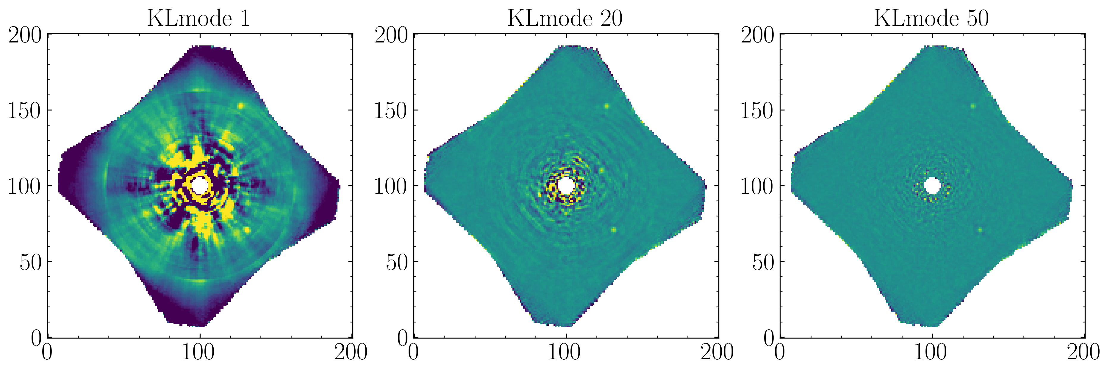
Running the tutorial on the example dataset produces the following PSF subtracted, collapsed images at each KL mode. Planet HR8799 c and d (upper right and lower right of the star, respectively) is already barely visible at 1 KLmode, and all three planets become clearly visible at 20 and 50 KLmodes.
Forward-Model Astrometry and Photometry
Once we have a detection and a known approximate location for the companion of interest, we can use forward modeling to model the companion PSF and fit for the astrometry and photometry. For a more detailed description of forward modeling and fitting for astrometry and photometry, please refer to Foward-Model Astrometry and Photometry.
You can run the forward modeled reduction with the following code.
import pyklip.fm as fm
import pyklip.fmlib.fmpsf as fmpsf

fm_outpath = '/path/to/forward/model/output'
prefix = 'object_name-fmpsf' # fileprefix for the output files

# setup FM guesses, change these to the numbers suited for your data.
# radius from primary star centroid in pixels
guesssep = 58.59
# position angle in degrees
guesspa = 333.16
guessflux = 2e-4 # in units of contrast to the host star
star_type = 'F8V'
guessspec = your_spectrum # should be 1-D array with number of elements = np.size(np.unique(dataset.wvs))

# since we now already know where the companion is roughly, we only have to reduce the region around the companion
# annuli and subsections can be specified as pixel and radian boundaries, respectively, instead of as integers.
annuli = [[guesssep-15, guesssep+15]] # one annulus centered on the planet
phi_section_size = 30 / guesssep # radians
subsections = [[np.radians(guesspa) - phi_section_size / 2.,
                np.radians(guesspa) + phi_section_size / 2.]] # one section centered on the planet
padding = 0 # we are not padding our zones
So far the reduction is identical to Basic KLIP Tutorial with GPI, except initializing data using the CHARIS module instead of the GPI module. The next code block sets up CHARIS instrumental psf models and flux normalization, which differs from pyKLIP’s general tutorial. The instrumental psf models are generated using the previously mentioned “satellite spots”. We generate psf stamps using the positions of the satellite spots measured in the image registration step, subtract the background from the central star’s halo, and then average the stamps over the (usually) four spots in each frame as well as over exposures. As a result, we obtain one psf model for each wavelength.
We then need to set the flux conversion for CHARIS that converts the psf models we just generated to the flux of the unocculted star. Since the psf models are generated from satellite spots, our flux conversion will be the flux ratios between the unocculted star and the satellite spots. The fluxes of the satellite spots scale as \(\propto A^2\lambda ^2\), where A is the amplitude of the diffractive grid and \(\lambda\) is the wavelength. The CHARIS module has, as a class constant, a reference spot-to-star contrast of \(2.72 \times 10^{-3} \pm 1.3 \times 10^{-4}\) at a grid amplitude of 0.25nm and a wavelength of 1.55 microns, which can then be scaled to all CHARIS wavelengths depending on the grid amplitude and the CHARIS bandpass. This reference flux ratio comes from measurements of an internal source over a narrow bandpass in Summer 2017, reported in Thayne et al.. The following code block generates the psf models and sets up the scaling that converts the psf models to the flux of the central star: \(F_{star} = F_{psf\;model} \times flux\;conversion\)
Note
Separate tests of the satellite spot to central star contrast performed on difference dates showed disagreements, suggesting that this flux ratio is not stable over time, and the results from a test closest to the date when the science data is taken should be used. Currently, there is one other measurement taken in Fall 2018 that gives a contrast of \(2.94 \times 10^{-3}\), an ~8% increase compared to 2017’s measurement. Some new pending calibration results suggest that this contrast has changed again since late 2021.
# generate a background-subtracted satellite spot PSFs with shape (nwv, boxsize, boxsize), averaged over exposures
boxsize = 15
dataset.generate_psfs(boxrad=boxsize // 2)

# sets up the contrast to data number conversion, further explained after this code block
wvs = np.unique(dataset.wvs) # in microns
dataset_gridamp = float(dataset.prihdrs[0]['X_GRDAMP'])
star_to_spot_ratio = 1. / ((dataset_gridamp / dataset.ref_spot_contrast_gridamp) ** 2
                           * dataset.ref_spot_contrast * dataset.ref_spot_contrast_wv ** 2 / (wvs ** 2))
flux_conversion = np.tile(star_to_spot_ratio, (dataset.input.shape[0]//22))
Now we are ready to run the forward modeling reduction:
fm_class = fmpsf.FMPlanetPSF(dataset.input.shape, numbasis, guesssep, guesspa, guessflux, dataset.psfs,
                             np.unique(dataset.wvs), flux_conversion, star_spt=star_type, spectrallib=guessspec)

fm.klip_dataset(dataset, fm_class, mode=mode, outputdir=fm_outpath, fileprefix=prefix, numbasis=numbasis,
                maxnumbasis=maxnumbasis, annuli=annuli, subsections=subsections, padding=padding,
                movement=movement, time_collapse='weighted-mean')
We can then use our forward models and the klipped data to measure astrometry and photometry of a detected companion. For details on fitting astrometry and photometry: please refer to Foward-Model Astrometry and Photometry.
Spectral Extraction
Once you have detected and fitted for the astrometry of the companion in previous sections, you now have the information required for spectral extraction, which is done using the extractSpec module in the forward modeling lilbrary.
The example below extracts a spectrum with shape (len(numbasis), number of wavelength channels) in units of contrast to
the satellite spot psfs dataset.psfs.
import pyklip.fmlib.extractSpec as es

exspec_outpath = '/path/to/extracted/spectrum/output'
prefix = 'object_name-fmspect' # fileprefix for the output files

# use the known planet separation and position angle,
# for example, use the measurements from the forward-model fitted astrometry
planet_sep = 58.59 # companion separation in pixels
planet_pa = 333.16 # companion position angle in degrees
planet_stamp_size = 10 # how big of a stamp around the companion in pixels, stamp will be stamp_size**2 pixels
stellar_template = None # a stellar template spectrum, if you want

# reduction parameters
numbasis = np.array([5, 20])
maxnumbasis = 150
mode = 'ADI+SDI'
annuli=[[planet_sep-planet_stamp_size, planet_sep+planet_stamp_size]]
phi_section_size = 2 * planet_stamp_size / planet_sep # radians
subsections=[[np.radians(planet_pa) - phi_section_size / 2.,
              np.radians(planet_pa) + phi_section_size / 2.]]
movement = 2

# generate a background-subtracted satellite spot PSFs with shape (nwv, boxsize, boxsize), averaged over exposures
boxsize = 15
dataset.generate_psfs(boxrad=boxsize//2)

fm_class = es.ExtractSpec(dataset.input.shape,
                          numbasis,
                          planet_sep,
                          planet_pa,
                          dataset.psfs,
                          np.unique(dataset.wvs),
                          stamp_size = planet_stamp_size)


fm.klip_dataset(dataset, fm_class,
                mode=mode,
                fileprefix=prefix,
                annuli=annuli,
                subsections=subsections,
                movement=movement,
                numbasis=numbasis,
                maxnumbasis=maxnumbasis,
                spectrum=stellar_template,
                outputdir=exspec_outpath, time_collapse='weighted-mean')

# If you want to scale your spectrum by a calibration factor:
units = "scaled"
scaling_factor = your_calibration_factor
#e.g. you could set scaling_factor to the star_to_spot_ratio variable in the previous section, which will convert
# the extracted spectrum from units of contrast to the satellite spot PSF to units of data number
# otherwise, the defaults are:
units = "natural" # (default) returned relative to input PSF model

fmout_nanzero = np.copy(dataset.fmout)
fmout_nanzero[np.isnan(fmout_nanzero)] = 0.
exspect, fm_matrix = es.invert_spect_fmodel(fmout_nanzero, dataset, units=units, scaling_factor=scaling_factor,
                                            method='leastsq')

np.savetxt(os.path.join(exspec_outpath, 'extracted_spectrum.txt'), exspect)
np.save(os.path.join(exspec_outpath, 'fm_matrix.npy'), fm_matrix)
Spectral Calibration
Finally, we calibrate the extracted contrast spectrum to physical units. The spectrum extracted in the previous section
is in units of contrast relative to our psf models at each wavelength dataset.psfs. To convert this to the spectrum
of the companion in real physical units, we need the stellar model spectrum for the host star, the observed magnitude
of the host star, and the contrast between the unocculted host star and our psf models. For the stellar models,
we use the The Castelli AND Kurucz 2004 Stellar Atmosphere Models
library implemented in the pysynphot package for
this tutorial. However, the user is free to use other models of their choosing. The calibration can be expressed as:
where \(\frac{F_{companion}}{F_{spot}}\) is the extracted spectrum from Spectral Extraction,
\(\frac{F_{spot}}{F_{star}}\) has been explained and defined in Forward-Model Astrometry and Photometry as star_to_spot_ratio,
which we re-use below, and \(F_{star}\) is calibrated from the stellar model of the host star type and the observed
magnitude of the host star.
First, we read in the extracted spectrum from the previous section, and convert the contrast spectrum relative to the satellite spots into the contrast spectrum relative to the host star:
import pyklip.spectra_management as klip_spectra
import pysynphot

fm_spec_path = '/path/to/extracted_spectrum.txt'
exspec = np.genfromtxt(os.path.join(fm_spec_path, 'extracted_spectrum.txt'))

# ensure extracted spectrum has shape (number of different KL modes, nwv), even if there is only one KL-mode
# this ensures consistent formatting later on
if len(exspec.shape) == 1:
    exspec = np.array([exspec])

contrast_spectra = exspec / star_to_spot_ratio[np.newaxis, :]
Then, we specify the stellar parameters for the host star and interpolate the stellar model library:
band = 'H' # 2MASS bandpass, 'J', 'H', or 'Ks'
primary_star_mag = 5.280  # 2MASS H band observed magnitude for HR8799
primary_star_mag_error = 0.018 # 2MASS H band magnitude error for HR8799

# 3 spectral libraries available: 'ck04models', 'k93models', 'phoenix'
model_lib = 'ck04models'
temperature = 7200
metallicity = 0
log_g = 4.34
stellar_model = pysynphot.catalog.Icat(model_lib, temperature, metallicity, log_g)
stellar_model_wvs = stellar_model.wave[stellar_model.wave < 25000] * 1e-4 # in microns
stellar_model_fluxes = stellar_model.flux[stellar_model.wave < 25000]
We need to resample the stellar model at the CHARIS wavelength bins, this can be done using calibrate_star_spectrum
in klip.spectra_management.
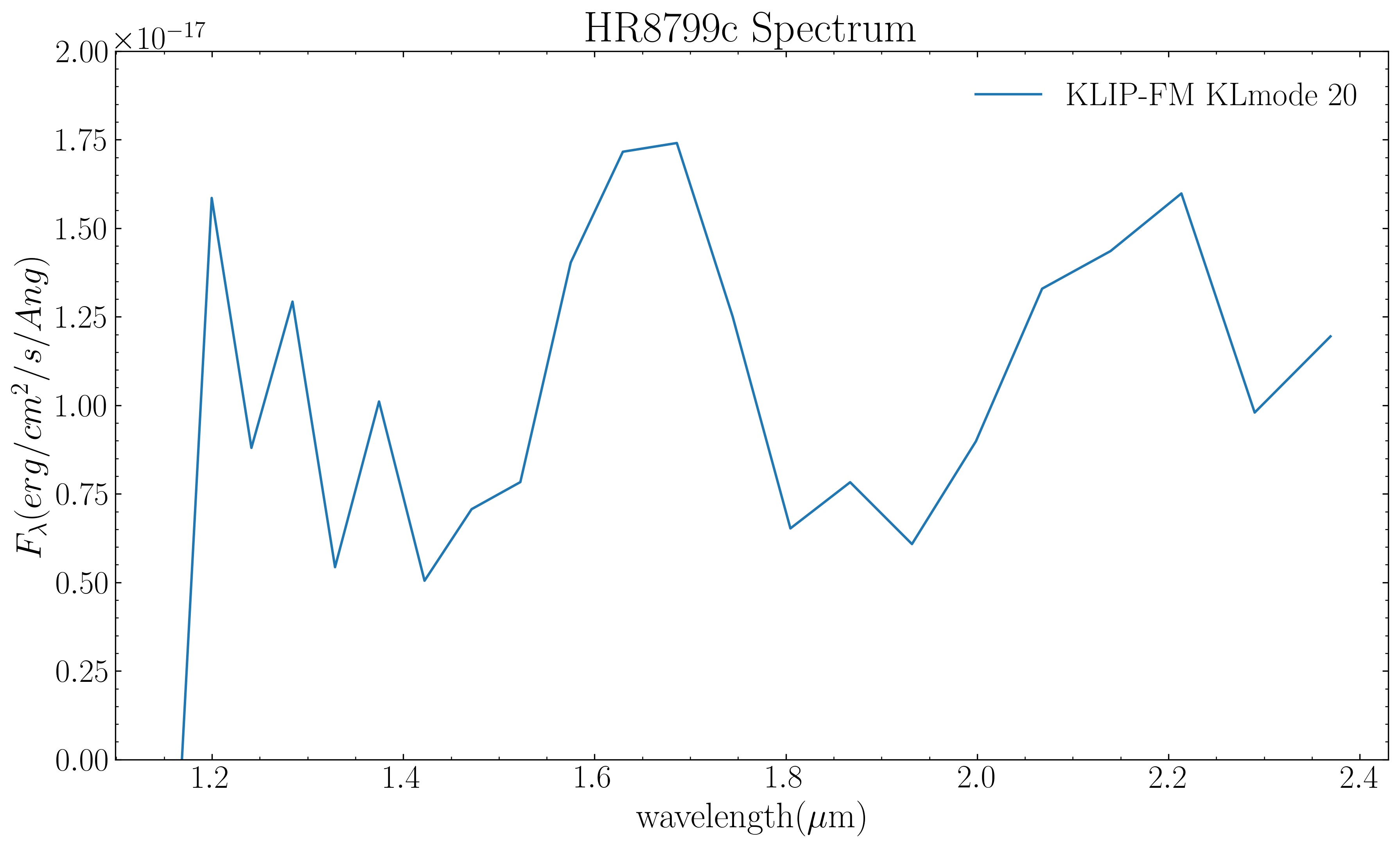
Finally, multiplying the contrast spectrum by the stellar model, we obtain the calibrated spectrum in flux density units. The extracted spectrum of planet c for the example dataset is shown here. Note that the quality is poor and quite different from the published spectrum of this planet because we are using a small subset of the full dataset for the tutorial.
# scale the stellar model to the observed magnitude and resample at the CHARIS wavelength bins
# return spectrum is the flux density in gaussian units (erg/cm^2/s/angstrom)
stellar_spectrum = klip_spectra.calibrate_star_spectrum(stellar_model_fluxes, stellar_model_wvs, 'H',
                                                        primary_star_mag, wvs * 1e4)

# finally we obtain the companion spectra in gaussian units for all KL-modes used in the reduction
companion_spectra = contrast_spectra * stellar_spectrum[np.newaxis, :]
Error Calculation
You can estimate the error bars and biases of the extracted spectrum by injecting synthetic sources and recovering them. The “Calculating Errorbars” section in Spectrum Extraction using extractSpec FM shows you how to do this.